Why Using Average Returns Can Mislead And Project Inflated Wealth Growth

Amit considered himself the luckiest investor alive. In June 1999, he made a bold decision—he would invest Rs 10 lakh in the Nifty 50 Total Return Index (TRI) and let it grow until December 2024. But Amit wasn’t like other investors. He had a secret weapon: perfect foresight.

He knew two things with absolute certainty: The average monthly return of the index would be 1.30 per cent. The volatility of those returns would be 6.30 per cent.

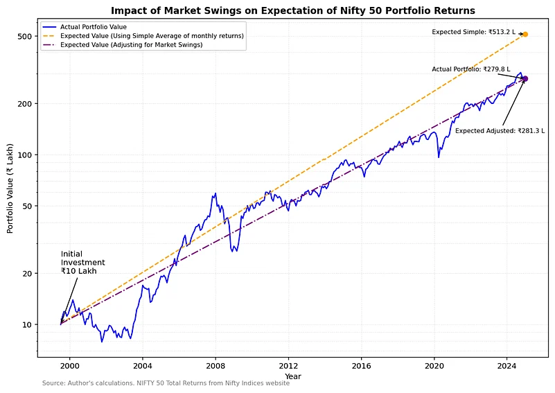
Armed with this crystal-clear vision, Amit confidently calculated that his investment would soar to Rs 513.2 lakh by 2024. As he pressed the invest button, he pictured himself reclining on a sunny Goan beach, sipping coconut water, and telling his friends, “Investing is easy if you understand the numbers!”

Fast forward 25 years, and December 2024 finally arrived. Excited to confirm his dream scenario, Amit logged in to his portfolio account—only to nearly spill his coffee. His portfolio was worth just Rs 279.80 lakh!

“How could this happen?” Amit muttered. “I knew the average return in advance! What went wrong?”

The culprit? Market volatility – a sneaky phenomenon that affects not just how investments grow, but how much they grow. Let’s unpack Amit’s story and see what it teaches us.

What Is Volatility?

Volatility is a measure of how much an investment’s returns fluctuate over time. Think of it as the mood swings of the market – some months are euphoric with double-digit gains, while others are turbulent with steep losses.

For Amit, the average monthly return of the Nifty 50 was 1.30 per cent, but that’s just one piece of the puzzle. Over 25 years, returns didn’t arrive neatly at 1.30 per cent every month. Some months soared far higher, while others plummeted deep into the red.

The return Amit ultimately saw in his portfolio wasn’t the simple average – it’s the compounded growth of his money over time, also known as the geometric return. This is what investors experience in reality.

Understanding volatility is useful, but we also need to consider how returns behave over time. This brings us to the concept of distributions.

Distributions: Beyond Averages

Returns, like many natural phenomena, follow a distribution – a way of describing all possible outcomes and how often they occur. The “average” return (mean) is just the middle of this distribution, while volatility measures how much the data spreads around this average.

Relying on averages alone is like describing a T20 cricket match by only stating the average runs scored in the innings. Adding volatility gives more context, such as mentioning the run rate and wickets.

But even this isn’t enough, because it still summarises the entire match into a single set of numbers, ignoring key moments like game-changing partnerships or collapses.

In Amit’s case, focusing only on the average return ignored the reality of how volatile swings shaped his actual portfolio value.

Volatility Drag: The Leaky Bucket

Here’s where volatility drag comes in. When returns fluctuate, the compounded or geometric return that investors experience is always lower than the arithmetic return (the simple average). The greater the volatility, the bigger this gap.

To see this in action, consider the chart below, which illustrates how market swings impact the expected value of a Nifty 50 portfolio over 25 years

A Simpler Way To Understand Volatility Drag

Imagine driving on a flat highway with a 60 km/hr speed limit. Without obstacles, your average speed is exactly 60 km/hr.

Now, picture yourself on a hilly road with sharp bends instead of a flat highway. While you might still reach 60 km/rh on straight stretches, you will need to slow down considerably on steep inclines or tight turns. Your actual speed at the end of the journey will be much lower – around 50 km/hr on average.

This is precisely what happens with investing:

• Arithmetic return is the 60 km/h highway speed.

• Volatility (market swings) are the hills and curves forcing you to slow down.

• Geometric return (actual return) is the lower average speed at which you reach your destination.

• Mathematically, volatility drag can be estimated using: 𝐺𝑒𝑜𝑚𝑒𝑡𝑟𝑖𝑐 𝑅𝑒𝑡𝑢𝑟𝑛≈𝐴𝑟𝑖𝑡ℎ𝑚𝑒𝑡𝑖𝑐 𝑅𝑒𝑡𝑢𝑟𝑛−𝑉𝑜𝑙𝑎𝑡𝑖𝑙𝑖𝑡𝑦22

• The higher the volatility, the greater the slowdown and bigger the gap between expected and realised wealth.

For Amit:

• The arithmetic return predicted Rs 513.2 lakh.

• Adjusting for volatility, the expected value dropped to Rs 281.3 lakh.

• The actual portfolio value was Rs 279.8 lakh – proof that volatility drag is real.

This is why understanding volatility is critical: it can make or break long-term investment expectations.

Diversification: Smoother Roads Lead To Better Outcomes

One way to reduce the impact of volatility drag is diversification. By spreading investments across asset classes, such as equities, bonds, and gold – you reduce overall volatility, even if individual assets are volatile.

Nobel Laureate and father of modern portfolio theory, Harry Markowitz, famously said, “Diversification is the only free lunch in investing”.

Here’s the counterintuitive part: A diversified portfolio may have lower average returns than a high-risk, high-return strategy. But because volatility drag is lower, the compounding effect is often higher.

The key insight? Even with lower average returns, a steady compounding effect often leads to better wealth accumulation over long horizons than a high-return, high-volatility strategy that experiences sharp losses.

This is not to say diversified portfolios won’t have drawdowns—they will. But they tend to provide smoother performance over longer time horizons and better real-world outcomes.

Why Simple Averages Are Misleading

Using simple averages to project investment outcomes can be dangerously misleading. Volatility drag and the characteristics of return distributions mean that projections based on arithmetic averages often overestimate future wealth.

As discussed in my paper Unbalanced Acts: Rethinking Naive Use of Historical Returns in Retirement Portfolio Strategies, ignoring these nuances can lead to flawed financial planning and unmet expectations.